The standard inner product of two vectors has some nice geometric properties. Given two vectors $ x, y \in \mathbb{R}^n$, where by $ x_i$ I mean the $ i$-th coordinate of $ x$, the standard inner product (which I will interchangeably call the dot product) is defined by the formula
$$\displaystyle \langle x, y \rangle = x_1 y_1 + \dots + x_n y_n$$This formula, simple as it is, produces a lot of interesting geometry. An important such property, one which is discussed in machine learning circles more than pure math, is that it is a very convenient decision rule.
In particular, say we’re in the Euclidean plane, and we have a line $ L$ passing through the origin, with $ w$ being a unit vector perpendicular to $ L$ (“the normal” to the line).
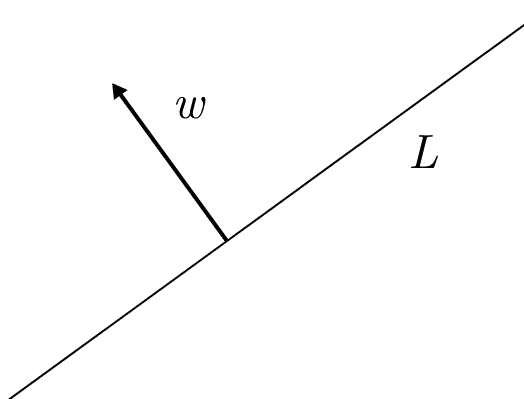
If you take any vector $ x$, then the dot product $ \langle x, w \rangle$ is positive if $ x$ is on the same side of $ L$ as $ w$, and negative otherwise. The dot product is zero if and only if $ x$ is exactly on the line $ L$, including when $ x$ is the zero vector.
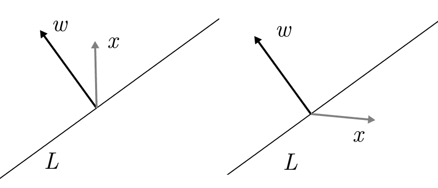
Left: the dot product of $ w$ and $ x$ is positive, meaning they are on the same side of $ w$. Right: The dot product is negative, and they are on opposite sides.
Here is an interactive demonstration of this property. Click the image below to go to the demo, and you can drag the vector arrowheads and see the decision rule change.
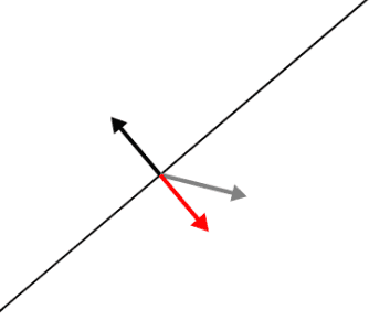
decision-rule
The code for this demo is available in a github repository.
It’s always curious, at first, that multiplying and summing produces such geometry. Why should this seemingly trivial arithmetic do anything useful at all?
The core fact that makes it work, however, is that the dot product tells you how one vector projects onto another. When I say “projecting” a vector $ x$ onto another vector $ w$, I mean you take only the components of $ x$ that point in the direction of $ w$. The demo shows what the result looks like using the red (or green) vector.
In two dimensions this is easy to see, as you can draw the triangle which has $ x$ as the hypotenuse, with $ w$ spanning one of the two legs of the triangle as follows:
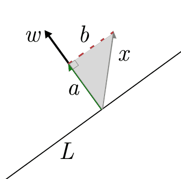
If we call $ a$ the (vector) leg of the triangle parallel to $ w$, while $ b$ is the dotted line (as a vector, parallel to $ L$), then as vectors $ x = a + b$. The projection of $ x$ onto $ w$ is just $ a$.
Another way to think of this is that the projection is $ x$, modified by removing any part of $ x$ that is perpendicular to $ w$. Using some colorful language: you put your hands on either side of $ x$ and $ w$, and then you squish $ x$ onto $ w$ along the line perpendicular to $ w$ (i.e., along $ b$).
And if $ w$ is a unit vector, then the length of $ a$—that is, the length of the projection of $ x$ onto $ w$—is exactly the inner product product $ \langle x, w \rangle$.
Moreover, if the angle between $ x$ and $ w$ is larger than 90 degrees, the projected vector will point in the opposite direction of $ w$, so it’s really a “signed” length.
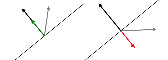
Left: the projection points in the same direction as $ w$. Right: the projection points in the opposite direction.
And this is precisely why the decision rule works. This 90-degree boundary is the line perpendicular to $ w$.
More technically said: Let $ x, y \in \mathbb{R}^n$ be two vectors, and $ \langle x,y \rangle $ their dot product. Define by $ \| y \|$ the length of $ y$, specifically $ \sqrt{\langle y, y \rangle}$. Define by $ \text{proj}_{y}(x)$ by first letting $ y’ = \frac{y}{\| y \|}$, and then let $ \text{proj}_{y}(x) = \langle x,y’ \rangle y’$. In words, you scale $ y$ to a unit vector $ y’$, use the result to compute the inner product, and then scale $ y$ so that it’s length is $ \langle x, y’ \rangle$. Then
Theorem: Geometrically, $ \text{proj}_y(x)$ is the projection of $ x$ onto the line spanned by $ y$.
This theorem is true for any $ n$-dimensional vector space, since if you have two vectors you can simply apply the reasoning for 2-dimensions to the 2-dimensional plane containing $ x$ and $ y$. In that case, the decision boundary for a positive/negative output is the entire $ n-1$ dimensional hyperplane perpendicular to $ y$ (the projected vector).
In fact, the usual formula for the angle between two vectors, i.e. the formula $ \langle x, y \rangle = \|x \| \cdot \| y \| \cos \theta$, is a restatement of the projection theorem in terms of trigonometry. The $ \langle x, y’ \rangle$ part of the projection formula (how much you scale the output) is equal to $ \| x \| \cos \theta$. At the end of this post we have a proof of the cosine-angle formula above.
Part of why this decision rule property is so important is that this is a linear function, and linear functions can be optimized relatively easily. When I say that, I specifically mean that there are many known algorithms for optimizing linear functions, which don’t have obscene runtime or space requirements. This is a big reason why mathematicians and statisticians start the mathematical modeling process with linear functions. They’re inherently simpler.
In fact, there are many techniques in machine learning—a prominent one is the so-called Kernel Trick—that exist solely to take data that is not inherently linear in nature (cannot be fruitfully analyzed by linear methods) and transform it into a dataset that is. Using the Kernel Trick as an example to foreshadow some future posts on Support Vector Machines, the idea is to take data which cannot be separated by a line, and transform it (usually by adding new coordinates) so that it can. Then the decision rule, computed in the larger space, is just a dot product. Irene Papakonstantinou neatly demonstrates this with paper folding and scissors. The tradeoff is that the size of the ambient space increases, and it might increase so much that it makes computation intractable. Luckily, the Kernel Trick avoids this by remembering where the data came from, so that one can take advantage of the smaller space to compute what would be the inner product in the larger space.
Next time we’ll see how this decision rule shows up in an optimization problem: finding the “best” hyperplane that separates an input set of red and blue points into monochromatic regions (provided that is possible). Finding this separator is core subroutine of the Support Vector Machine technique, and therein lie interesting algorithms. After we see the core SVM algorithm, we’ll see how the Kernel Trick fits into the method to allow nonlinear decision boundaries.
Proof of the cosine angle formula
Theorem: The inner product $ \langle v, w \rangle$ is equal to $ \| v \| \| w \| \cos(\theta)$, where $ \theta$ is the angle between the two vectors.
Note that this angle is computed in the 2-dimensional subspace spanned by $ v, w$, viewed as a typical flat plane, and this is a 2-dimensional plane regardless of the dimension of $ v, w$.
Proof. If either $ v$ or $ w$ is zero, then both sides of the equation are zero and the theorem is trivial, so we may assume both are nonzero. Label a triangle with sides $ v,w$ and the third side $ v-w$. Now the length of each side is $ \| v \|, \| w\|,$ and $ \| v-w \|$, respectively. Assume for the moment that $ \theta$ is not 0 or 180 degrees, so that this triangle is not degenerate.
The law of cosines allows us to write
$$\displaystyle \| v – w \|^2 = \| v \|^2 + \| w \|^2 – 2 \| v \| \| w \| \cos(\theta)$$Moreover, The left hand side is the inner product of $ v-w$ with itself, i.e. $ \| v – w \|^2 = \langle v-w , v-w \rangle$. We’ll expand $ \langle v-w, v-w \rangle$ using two facts. The first is trivial from the formula, that inner product is symmetric: $ \langle v,w \rangle = \langle w, v \rangle$. Second is that the inner product is linear in each input. In particular for the first input: $ \langle x + y, z \rangle = \langle x, z \rangle + \langle y, z \rangle$ and $ \langle cx, z \rangle = c \langle x, z \rangle$. The same holds for the second input by symmetry of the two inputs. Hence we can split up $ \langle v-w, v-w \rangle$ as follows.
$$\displaystyle \begin{aligned} \langle v-w, v-w \rangle &= \langle v, v-w \rangle – \langle w, v-w \rangle \\\ &= \langle v, v \rangle – \langle v, w \rangle – \langle w, v \rangle + \langle w, w \rangle \\\ &= \| v \|^2 – 2 \langle v, w \rangle + \| w \|^2 \\\ \end{aligned}$$Combining our two offset equations, we can subtract $ \| v \|^2 + \| w \|^2$ from each side and get
$$\displaystyle -2 \|v \| \|w \| \cos(\theta) = -2 \langle v, w \rangle, $$Which, after dividing by $ -2$, proves the theorem if $ \theta \not \in \{0, 180 \}$.
Now if $ \theta = 0$ or 180 degrees, the vectors are parallel, so we can write one as a scalar multiple of the other. Say $ w = cv$ for $ c \in \mathbb{R}$. In that case, $ \langle v, cv \rangle = c \| v \| \| v \|$. Now $ \| w \| = | c | \| v \|$, since a norm is a length and is hence non-negative (but $ c$ can be negative). Indeed, if $ v, w$ are parallel but pointing in opposite directions, then $ c < 0$, so $ \cos(\theta) = -1$, and $ c \| v \| = – \| w \|$. Otherwise $ c > 0$ and $ \cos(\theta) = 1$. This allows us to write $ c \| v \| \| v \| = \| w \| \| v \| \cos(\theta)$, and this completes the final case of the theorem.
$$\square$$Want to respond? Send me an email, post a webmention, or find me elsewhere on the internet.