CKKS — Polynomials, the Canonical Embedding, and Encoding

Table of Contents

In this tutorial series, I will introduce the CKKS homomorphic encryption scheme from the ground up, in rather intricate detail. Each article in this series corresponds to a pull request on a GitHub repository. The code for this article is in this pull request. Follow along by cloning the repository and checking out the code at the relevant commit.

This first article will cover some of the mathematical background necessary in the formulation of the CKKS encryption scheme, specifically the polynomial ring used in the most basic version of CKKS, and the canonical embedding used to encode cleartext messages as plaintexts.

This series will contain plenty of mathematics, but I may abbreviate some verbose definitions, especially those that I would expect to be familiar to readers of this blog (such as the formal definition of a ring). In other words, I’ll assume basic undergraduate mathematics familiarity, with some reminders. A good accompaniment for this series would be The Beginner’s Textbook for Fully Homomorphic Encryption by Ronny Ko, which complements this series in giving more complete (albeit terse) definitions, formulas, and proofs.

A brief history of CKKS

Some of the terms used in this section may make more sense if you’ve read my high-level technical overview of homomorphic encryption. We will re-cover all of this in detail in future articles.

The original CKKS homomorphic encryption scheme was introduced in the 2016 paper Homomorphic Encryption for Arithmetic of Approximate Numbers by Jung Hee Cheon, Andrey Kim, Miran Kim, and Yongsoo Song as a joint collaboration between Seoul National University and UC San Diego.¹ Its primary innovation was to handle approximate arithmetic on real or complex numbers, rather than prior schemes which only handled exact arithmetic on integers. This is relevant in contexts like neural network inference, where the calculations can be inexact and still useful. In particular, CKKS allows the inexactness of fixed-point arithmetic to coexist with the error introduced by the homomorphic encryption scheme itself.

After its initial publication, several followup papers made improvements to CKKS that elevated it to the state of the art. First, and most importantly, a bootstrapping procedure was found in 2018 that made CKKS “fully homomorphic.” Subsequent years saw a plethora of additional improvements and variants to CKKS bootstrapping. Experts would even say there are too many variants to keep track of.

The second major improvement was the introduction of the residue number system variant of CKKS in 2017. The original CKKS scheme used large integer arithmetic, in particular doing arithmetic modulo hundred-bit or even thousand-bit moduli. Using a residue number system (RNS) allows one to replace the (inherently serial) carry propagation required for large-precision arithmetic with parallel operations on vectors of 64-bit values.²

Combining RNS with bootstrapping produces what, in my view, is the “baseline” version of CKKS that most new works extend or use for contrast.

Plaintexts and a polynomial ring

The main setting for CKKS is a particular polynomial ring. We start with some ring $R$ of coefficients for the polynomials $R[x]$; sometimes $R$ will be the integers, reals, but more often it will be the field of integers modulo a prime.

CKKS is an encryption scheme, and in every encryption scheme there are three distinct spaces: the cleartext space, the plaintext space, and the ciphertext space.

Cleartexts describe the atomic message units (e.g., a vector of 32-bit integers of a fixed size). The user must decide how to split their larger program data into cleartext units, say, by chunking. Plaintexts describe preprocessing required to make a cleartext compatible with the encryption scheme. And ciphertexts are the form of the messages after they are encrypted.

I spell all this out because, while many encryption schemes don’t have major differences between cleartext and plaintext space, CKKS uses a sophisticated transformation. This article focuses purely on the conversion between the cleartext and plaintext space.

Fix a parameter $N$, a power of two, which will be used to define the polynomial ring. A CKKS cleartext is a vector of $N/2$ complex numbers.³ A CKKS plaintext is an element of the ring

As a reminder, the coefficients $\mathbb{Z}/Q\mathbb{Z}$ form the ring of integers with arithmetic done modulo $Q$. If $Q$ were a prime, this would form a field, but in most cases $Q$ is composite.

As a second reminder, the polynomial modulus converts the ring of polynomials mod $Q$ into a quotient ring where two polynomials $p(x)$ and $q(x)$ are equivalent if they have the same remainder when dividing by $x^N + 1$. Some features that are important for computation:

• Elements of this ring have degree bounded by $N-1$ (when choosing their minimal-degree coset representative). So a polynomial can be viewed as a vector of $N$ entries, the coefficients at degrees 0 to $N-1$.
• One can identify $x^N$ with $-1$, and this gives a baseline method to reduce larger polynomials to their canonical representative: take each coefficient at degree $k \geq N$ and add it with a sign flip to the coefficient at degree $k - N$.
• Because of the previous item, multiplying a polynomial in this ring by a monomial can be implemented by cyclically rotating the coefficient vector and sign-flipping the values that wrap around an odd number of times. This operation is also known as negacyclic rotation.

There are other important structures of this ring for cryptographic reasons.⁴ For one, the value of $N$ being a power of two ensures this polynomial forms a number field. I don’t want to go too deeply into Galois theory here, but the basic idea of a number field is that you start from the rational numbers $\mathbb{Q}$, pick a finite number of elements $\alpha_1, \dots, \alpha_r$ not in $\mathbb{Q}$ (in our case they will be complex roots of unity), and “add them” to $\mathbb{Q}$, forming an extension field $\mathbb{Q}(\alpha_1, \dots, \alpha_r)$ by also including all the derived quantities required to satisfy the field axioms (inverses, sums and products, sums of products, etc.).⁵ In order to be a number field, these elements need to have some finite algebraic formula that gets them back to zero. In other words, the degree of $\mathbb{Q}(\alpha_1, \dots, \alpha_r)$ as a $\mathbb{Q}$-vector space must be finite. The simplest example is $\mathbb{Q}(\sqrt{2})$, which has degree 2 because $\sqrt{2}$ is a root of the polynomial $x^2 - 2$.

Back to CKKS, the polynomial ring $(\mathbb{Z}/Q\mathbb{Z})[x] \Big / (x^N+1)$ is not obviously a number field. You have to do a bit of work to first identify $\mathbb{Z}[x] \Big / (x^N+1)$ with $K = \mathbb{Q}(\omega_{2N})$, where $\omega_{2N}$ is a primitive $2N$-th root of unity.⁶ Once you do, taking a quotient by $Q$ in the coefficients translates to a quotient ring $K / QK$. Another angle is to start from $\mathbb{Z}[x] / (x^N + 1)$, identify that as the ring of integers of the number field $\mathbb{Q}[x] / (x^N + 1) = \mathbb{Q}(\omega_{2N})$, and take a quotient by the modulus $Q$.

We will touch on this more later in the series. The choice of $N$ and $Q$ implies a particular structure of this quotient ring, which impacts how we implement various homomorphic operations. In particular, it affects the efficiency of the number theoretic transform. But for this article, what matters is mainly that the plaintexts are polynomials and that their coefficients are discrete. This implies two obstacles:

• We must transform a vector of complex numbers into a polynomial.
• We must discretize an inherently continuous quantity, complex numbers.

The canonical embedding

The tool that CKKS uses to solve both of these problems is called the canonical embedding. This term has a lot of abstract definitions in different parts of mathematics, but for our purposes the canonical embedding has a simple definition.

Definition: Let $N$ be a power of two, and let $p(x)$ be a polynomial in $\mathbb{C}[x] / (x^N + 1)$. Then the canonical embedding of $p(x)$ in $\mathbb{C}^N$ is the vector of evaluations of $p(x)$ at the roots of $x^N + 1$. In particular, for a primitive $2N$-th root of unity $\omega = e^{2 \pi i / (2N)} = e^{\pi i / N}$ (which generates the roots of $x^N + 1$), the canonical embedding of $p(x)$ is the vector

Define the canonical embedding $\sigma_N$ to map polynomials to their evaluations at the odd powers of the complex $2N$-th roots of unity.⁷

Let’s prove some properties of the canonical embedding.

Homomorphism: Evaluating a polynomial at a fixed value is a homomorphism with respect to addition and scaling of the polynomials ($(p+q)(x) = p(x) + q(x)$ by definition), and the same is true componentwise for different evaluations, so $\sigma_N$ is a homomorphism from $\mathbb{C}[x] / (x^N + 1) \to \mathbb{C}^N$.

Well-defined: Let $p(x)$ and $q(x)$ have the property that $x^N + 1$ divides $p(x) - q(x)$. Then for any root $r$ of $x^N + 1$ we have $p(r) - q(r) = 0$. Hence,

Conjugate symmetry when coefficients are real: when the input $p(x)$ to the canonical embedding happens to have real coefficients, it holds that $p(x)$ commutes with complex conjugation of its inputs, i.e., $p(\overline{x}) = \overline{p(x)}$. Combine this with the fact that the roots of $x^N + 1$ come in conjugate pairs:

And you get that, in this special case of real coefficients, the canonical embedding has a special conjugate symmetry: the second half of the vector’s entries are the reversed-complex conjugates of the first half.

This property has been named the “Hermitian” property, and given a name: $\mathbb{H}^N$ is defined as the set of complex vectors in $\mathbb{C}^N$ whose second half is the reversed-complex conjugates of the first half.

You might think that, because the second half of $\mathbb{H}^N$ is uniquely determined by the first half, that $\mathbb{H}^N$ is isomorphic to $\mathbb{C}^{N/2}$. You’d be right, but you have to be careful. Because despite having complex-valued entries, $\mathbb{H}^N$ is not a vector space over $\mathbb{C}$ at all. Scalar multiplication by a complex number does not preserve the conjugate symmetry. It only does so if the scalar is real. So $\mathbb{H}^N$ and $\mathbb{C}^{N/2}$ are isomorphic, but only as $\mathbb{R}$-vector spaces.

The above limitation is no problem, however, because we actually want our input vectors to be real-valued polynomials (so we can round them to integer-coefficient plaintexts). This leads us to the next fact, which is the converse of the “Conjugate symmetry when coefficients are real” fact above.

Proposition: Let $v \in \mathbb{H}^N$, and $\sigma_N : \mathbb{C}[x] \Big / (x^N + 1) \to \mathbb{C}^N$ be the canonical embedding. Then $\sigma_N^{-1}(v) \in \mathbb{R}[x] \Big / (x^N + 1)$, i.e., has real-valued coefficients.

Finally, the last property, which I will not prove here (see Appendix C of Damgård-Pastro-Smart-Zakarias), relates the geometry of the input and output of the canonical embedding. This is useful when analyzing the noise growth of CKKS ciphertexts. In fact, as far as I can tell this was one of the core reasons the original CKKS authors bothered with all this machinery:

Proposition: Fix $N$ and let $\sigma = \sigma_N$ be the canonical embedding as defined above. Let $\left \| x \right \|$ denote the infinity-norm of $x$ (the magnitude of the largest component). Then for all $p(x), q(x)$,

Moreover, there is a constant $c$ (depending only on $N$) such that for every $p(x)$,

These facts allow one to measure the growth of polynomial error in the CKKS scheme by analyzing the growth of the canonical embeddings. We will come back to that topic in future articles.

Implementing the canonical embedding and its inverse

In this section we’ll implement the canonical embedding and its inverse in Python. Reminder, the code can be found in commit 386f028 of this pull request for the overall tutorial series.

Because the canonical embedding involves evaluating a polynomial at a set of complex roots of unity, we naturally turn to the Fast Fourier Transform. See “Polynomial Multiplication Using the FFT” and “Negacyclic Polynomial Multiplication for more details of why this is a good approach. In particular, the canonical embedding and its inverse reduce to particular invocations of fft and ifft.

We start with a simple Polynomial class that wraps the coefficients and $N$.

class Polynomial:
    """A univariate polynomial with a ring modulus x^N + 1."""

    def __init__(self, coefficients: np.ndarray, modulus_degree: int):
        self.coefficients = coefficients
        self.modulus_degree = modulus_degree
        # ... <validations> ...

    # ... __eq__, __repr__, etc. ...

The above doesn’t include any actual polynomial operators yet, since these functions will mutate the underlying coefficients directly.

def canonical_embedding(poly: Polynomial) -> np.ndarray:
    """Computes the canonical embedding of a polynomial."""
    poly_coeffs = poly.coefficients
    N = poly.modulus_degree

    # 2N-point FFT evaluates at all 2N-th roots: omega^0, omega^1, ...,
    # omega^{2N-1}. But return only the odd entries for the primitive roots.
    padded = np.concatenate([poly_coeffs, np.zeros(N)])
    fft_result = np.fft.ifft(padded) * (2 * N)
    return fft_result[np.arange(1, 2 * N, 2)]

This method is slightly inefficient: to get the numpy.fft.fft/ifft functions to correspond to evaluations at $2N$-th roots of unity, we need to have a vector of length $2N$ as input. Then afterward to get the odd evaluations, we need to filter by the appropriate range.

To be more efficient, production CKKS implementations implement a custom FFT routine here that avoids this extra work in two ways: first by operating on the odd powers directly, and second taking advantage of the additional conjugate symmetry of the odd powers. For one such reference, see the FFTSpecial invocation in OpenFHE’s CKKS encoding routine, which implements Algorithm 1 of Chen-Chillotti-Song 2018.⁸

Commit 386f028 also includes a more direct implementation using a matrix-vector multiplication by the Vandermonde matrix. In the tests for this commit, we include equivalence testing of the two methods.

Encoding and decoding

With all the hard work done, we turn to encoding. The inverse of the canonical embedding allows us to map a complex (Hermitian) vector to a polynomial with real coefficients. However, to get a polynomial with integer coefficients (our desired plaintext space), we need to round. That raises the question of precision.

CKKS’s solution is the same as traditional fixed-point arithmetic. That is, we choose a scaling factor $\Delta$, and multiply the polynomial’s coefficients by $\Delta$ before rounding to the nearest integer. The message can be recovered by dividing by $\Delta$.

Fixed-point arithmetic will have major implications for CKKS. Specifically, it introduces an application-dependent decision for how to set parameters. Applications that can afford to be a bit less precise (like neural networks) can use smaller scaling factors, which leads to more efficient programs. We will return to this topic in fine detail later. For now, it gives us our final encoding algorithm:

1. Apply the inverse canonical embedding.
2. Multiply by the scale $\Delta$.
3. Round to the nearest integer mod $Q$.

Because scaling by $\Delta$ is followed by rounding mod $Q$, the choice of $Q$ implies a limit to the choice of $\Delta$: the scaled coefficients after step 2 cannot exceed $Q/2$, or else they will wrap around mod $Q$ and the original value will be lost.

The code in commit 2410f9d demonstrates this.

First we have a dataclass for parameters

Cleartext = np.ndarray
Plaintext = Polynomial

@dataclass(frozen=True)
class EncodingParams:
    scale: float
    poly_modulus_degree: int

Then encoding is

def encode(message: Cleartext, params: EncodingParams) -> Plaintext:
    """Encode a vector of complex numbers into a plaintext polynomial."""
    # Pad with zeros up to N / 2
    num_zeros = params.poly_modulus_degree // 2 - message.shape[0]
    if num_zeros:
        message = np.concatenate(
            [message, np.zeros(num_zeros, dtype=message.dtype)]
        )

    # Concat with flipped conjugate to make Hermitian
    hermitian_msg = np.concatenate(
        [message, np.flip(np.conjugate(message))]
    )

    # Result of inverse canonical_embedding is guaranteed to
    # be real-valued.
    polynomial = inverse_canonical_embedding(hermitian_msg)
    rounded_scaled_coeffs = np.round(
        np.real(polynomial.coefficients) * params.scale
    )
    return Polynomial(rounded_scaled_coeffs, params.poly_modulus_degree)

Similarly, decoding divides by the scale, applies the canonical embedding, and then returns the first $N/2$ slots.

def decode(plaintext: Plaintext, params: EncodingParams) -> Cleartext:
    """Decode a CKKS plaintext into a vector of complex numbers."""
    scale_removed = Polynomial(
        coefficients=plaintext.coefficients / params.scale,
        modulus_degree=plaintext.modulus_degree,
    )
    unembedded = canonical_embedding(scale_removed)
    return unembedded[: params.poly_modulus_degree // 2]

Investigating precision

To understand the precision loss of CKKS encoding in a bit more detail, let’s plot it.

Commit 0df5650 provides the code, and for $N=32$ with scaling factors ranging from $2$ to $2^{40}$ (the latter is a typical CKKS scaling factor seen in the wild), this is the plot of absolute and relative errors.

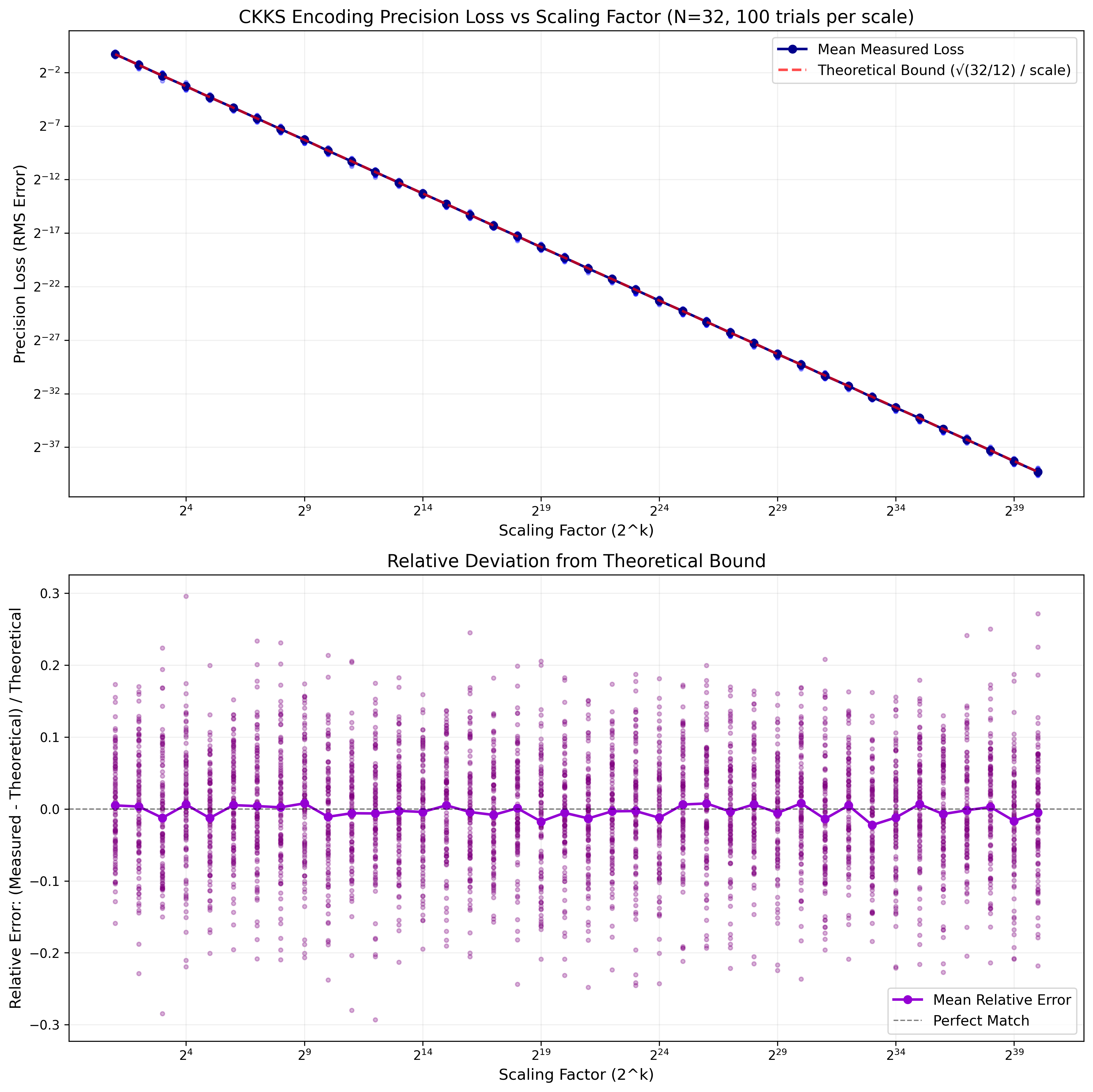
The top plot shows that absolute precision scales linearly with the scaling factor. The bottom plot shows the relative deviation from the theoretical bound, and even for a smallish $N=32$ the fit is pretty good. The “theoretical” line plotted corresponds to the average expected root-mean-squared precision loss, by following heuristic reasoning.

For $N$ random values, rounding introduces a uniform error in $[-0.5, 0.5]$ for each of the coefficients. Decoding sums these errors, and the resulting distribution is Gaussian with mean roughly $\sqrt{N}$.

We can also plot this as $N$ grows (commit 090147f).

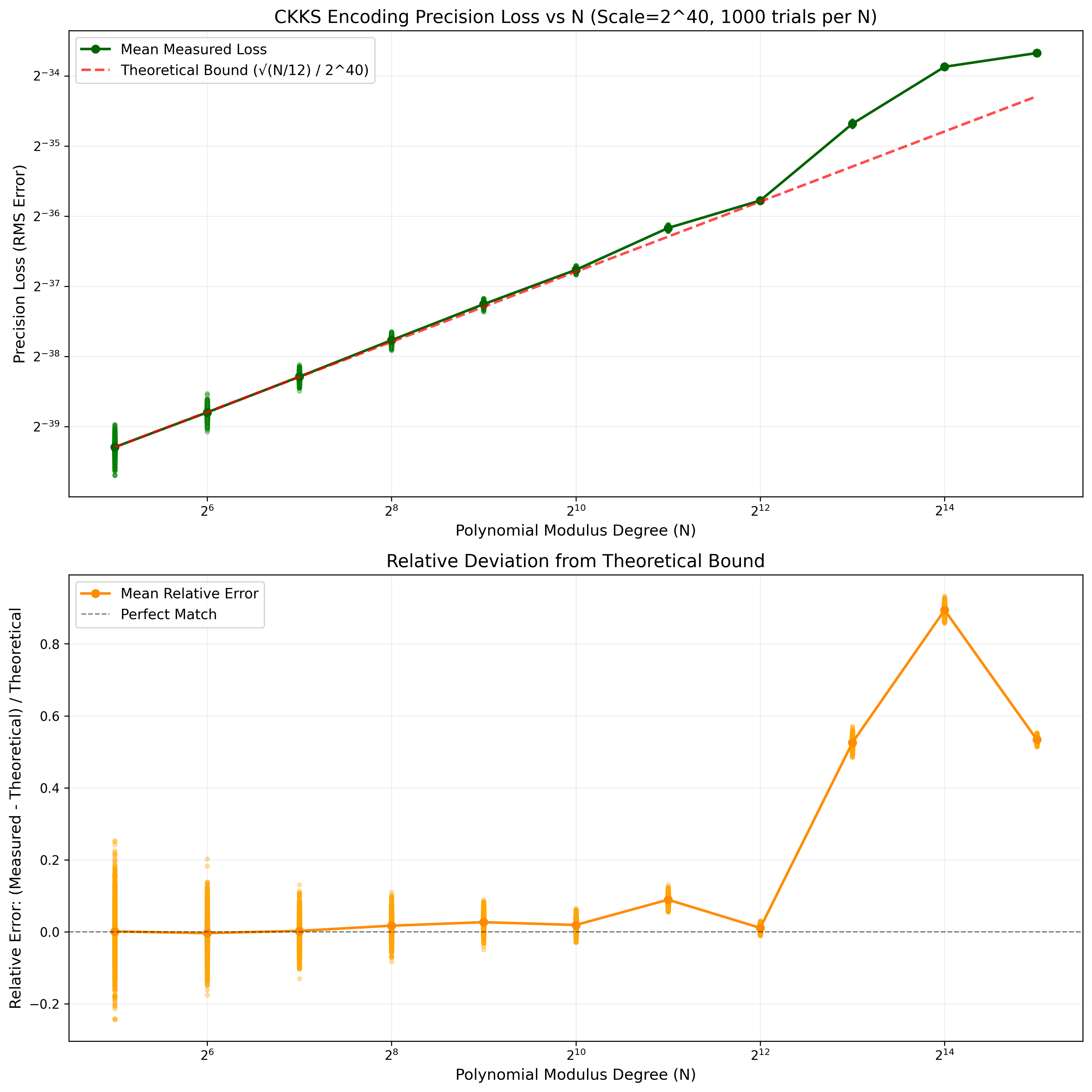
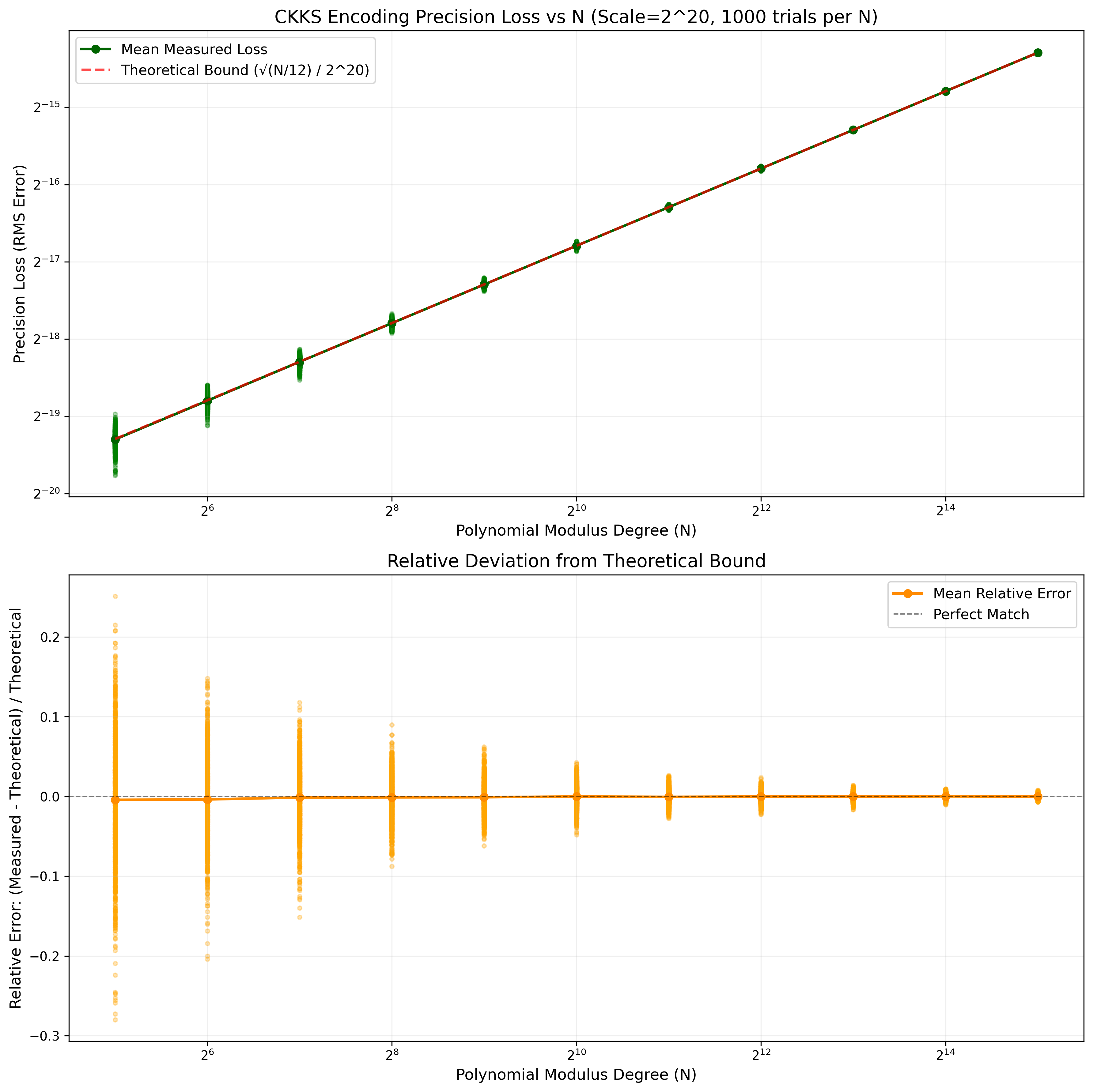
The theoretical bound still holds, except that when $N$ is sufficiently large (and when the scaling factor is sufficiently large), then, as best I can tell, the floating point errors in the FFT routine itself are of comparable magnitude to the precision loss due to rounding, which would explain the positive bias in error. At least, if I reduce the scaling factor to $2^{20}$, this positive bias disappears:

Wrapping it up

Recapping, the two obstacles we faced at the start of the article were:

• We must transform a vector of complex numbers into a polynomial.
• We must discretize an inherently continuous quantity, complex numbers.

The canonical embedding solves the first obstacle by providing an isomorphism between vectors of complex numbers and polynomials. The use of fixed-point arithmetic and a scaling factor solves the second.

While CKKS encoding does introduce errors in its encoding process, the standard intended application⁹ of CKKS is to machine learning inference. In this context, programs are naturally tolerant of error, and the encoding error is a small one-time cost. As we will see throughout the rest of the tutorial, encoding error will become dominated by rescaling and bootstrapping noise. But either way, it’s important not to forget about this source of error.

Acknowledgements

Thanks to Asra Ali, Edward Chen, Jianming Tong, and Hongren Zheng for feedback on a draft of this article.