Computing Homology

Update: the mistakes made in the code posted here are fixed and explained in a subsequent post (one minor code bug was fixed here, and a less minor conceptual bug is fixed in the linked post).

In our last post in this series on topology, we defined the homology group. Specifically, we built up a topological space as a simplicial complex (a mess of triangles glued together), we defined an algebraic way to represent collections of simplices called chains as vectors in a vector space, we defined the boundary homomorphism ${\partial }_k$ as a linear map on chains, and finally defined the homology groups as the quotient vector spaces

${\displaystyle H_k(X)=\frac{\text{ker}{\partial }_k}{\text{im}{\partial }_{k+1}}}$.

The number of holes in $X$ was just the dimension of this quotient space.

In this post we will be quite a bit more explicit. Because the chain groups are vector spaces and the boundary mappings are linear maps, they can be represented as matrices whose dimensions depend on our simplicial complex structure. Better yet, if we have explicit representations of our chains by way of a basis, then we can use row-reduction techniques to write the matrix in a standard form.

Of course the problem arises when we want to work with two matrices simultaneously (to compute the kernel-mod-image quotient above). This is not computationally any more difficult, but it requires some theoretical fiddling. We will need to dip a bit deeper into our linear algebra toolboxes to see how it works, so the rusty reader should brush up on their linear algebra before continuing (or at least take some time to sort things out if or when confusion strikes).

Without further ado, let’s do an extended example and work our ways toward a general algorithm. As usual, all of the code used for this post is available on this blog’s Github page.

Two Big Matrices

Recall our example simplicial complex from last time.

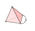
We will compute $H_1$ of this simplex (which we saw last time was $\mathbb{Q}$) in a more algorithmic way than we did last time.

Once again, we label the vertices 0-4 so that the extra “arm” has vertex 4 in the middle, and its two endpoints are 0 and 2. This gave us orientations on all of the simplices, and the following chain groups. Since the vertex labels (and ordering) are part of the data of a simplicial complex, we have made no choices in writing these down.

Now given our known definitions of ${\partial }_k$ as an alternating sum from last time, we can give a complete specification of the boundary map as a matrix. For ${\partial }_1$, this would be

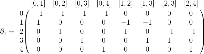
where the row labels are the basis for $C_0(X)$ and the column labels are the basis for $C_1(X)$. Similarly, ${\partial }_2$ is

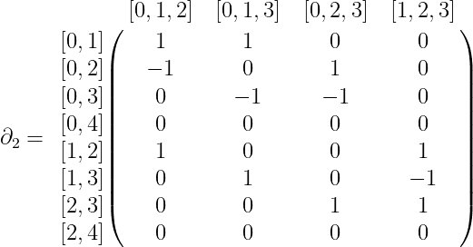
The reader is encouraged to check that these matrices are written correctly by referring to the formula for $\partial$ as given last time.

Remember the crucial property of $\partial$, that ${\partial }^2={\partial }_k{\partial }_{k+1}=0$. Indeed, the composition of the two boundary maps just corresponds to the matrix product of the two matrices, and one can verify by hand that the above two matrices multiply to the zero matrix.

We know from basic linear algebra how to compute the kernel of a linear map expressed as a matrix: column reduce and inspect the columns of zeros. Since the process of row reducing is really a change of basis, we can encapsulate the reduction inside a single invertible matrix $A$, which, when left-multiplied by $\partial$, gives us the reduced form of the latter. So write the reduced form of ${\partial }_1$ as ${\partial }_{1}A$.

However, now we’re using two different sets of bases for the shared vector space involved in ${\partial }_1$ and ${\partial }_2$. In general, it will no longer be the case that ${\partial }_{k}A{\partial }_{k+1}=0$. The way to alleviate this is to perform the “corresponding” change of basis in ${\partial }_{k+1}$. To make this idea more transparent, we return to the basics.

Changing Two Matrices Simultaneously

Recall that a matrix $M$ represents a linear map between two vector spaces $f:V\to W$. The actual entries of $M$ depend crucially on the choice of a basis for the domain and codomain. Indeed, if $v_i$ form a basis for $V$ and $w_j$ for $W$, then the $k$-th column of the matrix representation $M$ is defined to be the coefficients of the representation of $f(v_k)$ in terms of the $w_j$. We hope to have nailed this concept down firmly in our first linear algebra primer.

Recall further that row operations correspond to changing a basis for the codomain, and column operations correspond to changing a basis for the domain. For example, the idea of swapping columns $i,j$ in $M$ gives a new matrix which is the representation of $f$ with respect to the (ordered) basis for $V$ which swaps the order of $v_i,v_j$. Similar things happen for all column operations (they all correspond to manipulations of the basis for $V$), while analogously row operations implicitly transform the basis for the codomain. Note, though, that the connection between row operations and transformations of the basis for the codomain are slightly more complicated than they are for the column operations. We will explicitly see how it works later in the post.

And so if we’re working with two maps $A:U\to V$ and $B:V\to W$, and we change a basis for $V$ in $B$ via column reductions, then in order to be consistent, we need to change the basis for $V$ in $A$ via “complementary” row reductions. That is, if we call the change of basis matrix $Q$, then we’re implicitly sticking $Q$ in between the composition $BA$ to get $(BQ)A$. This is not the same map as $BA$, but we can make it the same map by adding a $Q^{-1}$ in the right place:

Indeed, whenever $Q$ is a change of basis matrix so is $Q^{-1}$ (trivially), and moreover the operations that $Q$ performs on the columns of $B$ are precisely the operations that $Q^{-1}$ performs on the rows of $A$ (this is because elementary row operations take different forms when multiplied on the left or right).

Coming back to our boundary operators, we want a canonical way to view the image of ${\partial }_{k+1}$ as sitting inside the kernel of ${\partial }_k$. If we go ahead and use column reductions to transform ${\partial }_k$ into a form where the kernel is easy to read off (as the columns consisting entirely of zeroes), then the corresponding row operations, when performed on ${\partial }_{k+1}$ will tell us exactly the image of ${\partial }_{k+1}$ inside the kernel of ${\partial }_k$.

This last point is true precisely because $\text{im}{\partial }_{k+1}\subset \text{ker}{\partial }_k$. This fact guarantees that the irrelevant rows of the reduced version of ${\partial }_{k+1}$ are all zero.

Let’s go ahead and see this in action on our two big matrices above. For ${\partial }_1$, the column reduction matrix is

${\displaystyle A=\left(\begin{array}{cccccccc}0& 1& 0& 0& 1& 1& 0& 0\\ 0& 0& 1& 0& -1& 0& 1& 1\\ 0& 0& 0& 1& 0& -1& -1& 0\\ -1& -1& -1& -1& 0& 0& 0& -1\\ 0& 0& 0& 0& 1& 0& 0& 0\\ 0& 0& 0& 0& 0& 1& 0& 0\\ 0& 0& 0& 0& 0& 0& 1& 0\\ 0& 0& 0& 0& 0& 0& 0& 1\end{array}\right)}$

And the product ${\partial }_{1}A$ is

${\displaystyle {\partial }_{1}A=\left(\begin{array}{cccccccc}1& 0& 0& 0& 0& 0& 0& 0\\ 0& 1& 0& 0& 0& 0& 0& 0\\ 0& 0& 1& 0& 0& 0& 0& 0\\ 0& 0& 0& 1& 0& 0& 0& 0\\ -1& -1& -1& -1& 0& 0& 0& 0\end{array}\right)}$

Now the inverse of $A$, which is the corresponding basis change for ${\partial }_2$, is

${\displaystyle A^{-1}=\left(\begin{array}{cccccccc}-1& -1& -1& -1& -0& -0& -0& -0\\ 1& 0& 0& 0& -1& -1& 0& 0\\ 0& 1& 0& 0& 1& 0& -1& -1\\ 0& 0& 1& 0& 0& 1& 1& 0\\ 0& 0& 0& 0& 1& 0& 0& 0\\ 0& 0& 0& 0& 0& 1& 0& 0\\ 0& 0& 0& 0& 0& 0& 1& 0\\ 0& 0& 0& 0& 0& 0& 0& 1\end{array}\right)}$

and the corresponding reduced form of ${\partial }_2$ is

${\displaystyle A^{-1}{\partial }_2=\left(\begin{array}{cccc}0& 0& 0& 0\\ 0& 0& 0& 0\\ 0& 0& 0& 0\\ 0& 0& 0& 0\\ 1& 0& 0& 1\\ 0& 1& 0& -1\\ 0& 0& 1& 1\\ 0& 0& 0& 0\end{array}\right)}$

As a side note, we got these matrices by slightly modifying the code from our original post on row reduction to output the change of basis matrix in addition to performing row reduction. It turns out one can implement column reduction as row reduction of the transpose, and the change of basis matrix you get from this process will be the transpose of the change of basis matrix you want (by $(AB{)}^{\text{T}}=(B^{\text{T}}{A}^{\text{T}})$). Though the code is particularly ad-hoc, we include it with the rest of the code used in this post on this blog’s Github page.

Now let’s inspect the two matrices ${\partial }_{1}A$ and $A^{-1}{\partial }_2$ more closely. The former has four “pivots” left over, and this corresponds to the rank of the matrix being 4. Moreover, the four basis vectors representing the columns with nonzero pivots, which we’ll call $v_1,v_2,v_3,v_4$ (we don’t care what their values are), span a complementary subspace to the kernel of ${\partial }_1$. Hence, the remaining four vectors (which we’ll call $v_5,v_6,v_7,v_8$) span the kernel. In particular, this says that the kernel has dimension 4.

On the other hand, we performed the same transformation of the basis of $C_1(X)$ for ${\partial }_2$. Looking at the matrix that resulted, we see that the first four rows and the last row (representing $v_1,v_2,v_3,v_4,v_8$) are entirely zeros and so the image of ${\partial }_2$ intersects their span trivially. and the remaining three rows (representing $v_5,v_6,v_7$) have nonzero pivots. This tells us exactly that the image of ${\partial }_2$ is spanned by $v_5,v_6,v_7$.

And now, the coup de grâce, the quotient to get homology is simply

And the dimension of the homology group is 1, as desired.

The General Algorithm

It is no coincidence that things worked out at nicely as they did. The process we took of simultaneously rewriting two matrices with respect to a common basis is the bulk of the algorithm to compute homology. Since we’re really only interested in the dimensions of the homology groups, we just need to count pivots. If the number of pivots arising in ${\partial }_k$ is $y$ and the number of pivots arising in ${\partial }_{k+1}$ is $z$, and the dimension of $C_k(X)$ is $n$, then the dimension is exactly

And it is no coincidence that the pivots lined up so nicely to allow us to count dimensions this way. It is a minor exercise to prove it formally, but the fact that the composition ${\partial }_k{\partial }_{k+1}=0$ implies that the reduced version of ${\partial }_{k+1}$ will have an almost reduced row-echelon form (the only difference being the rows of zeros interspersed above, below, and possibly between pivot rows).

As the reader may have guessed at this point, we don’t actually need to compute $A$ and $A^{-1}$. Instead of this, we can perform the column/row reductions simultaneously on the two matrices. The above analysis helped us prove the algorithm works, and with that guarantee we can throw out the analytical baggage and just compute the damn thing.

Indeed, assuming the input is already processed as two matrices representing the boundary operators with respect to the standard bases of the chain groups, computing homology is only slightly more difficult than row reducing in the first place. Putting our homology where our mouth is, we’ve implemented the algorithm in Python. As usual, the entire code used in this post is available on this blog’s Github page.

The first step is writing auxiliary functions to do elementary row and column operations on matrices. For this post, we will do everything in numpy (which makes the syntax shorter than standard Python syntax, but dependent on the numpy library).

import numpy

def rowSwap(A, i, j):
   temp = numpy.copy(A[i, :])
   A[i, :] = A[j, :]
   A[j, :] = temp

def colSwap(A, i, j):
   temp = numpy.copy(A[:, i])
   A[:, i] = A[:, j]
   A[:, j] = temp

def scaleCol(A, i, c):
   A[:, i] *= c*numpy.ones(A.shape[0])

def scaleRow(A, i, c):
   A[i, :] *= c*numpy.ones(A.shape[1])

def colCombine(A, addTo, scaleCol, scaleAmt):
   A[:, addTo] += scaleAmt * A[:, scaleCol]

def rowCombine(A, addTo, scaleRow, scaleAmt):
   A[addTo, :] += scaleAmt * A[scaleRow, :]

From here, the main meat of the algorithm is doing column reduction on one matrix, and applying the corresponding row operations on the other.

def simultaneousReduce(A, B):
   if A.shape[1] != B.shape[0]:
      raise Exception("Matrices have the wrong shape.")

   numRows, numCols = A.shape # col reduce A

   i,j = 0,0
   while True:
      if i >= numRows or j >= numCols:
         break

      if A[i][j] == 0:
         nonzeroCol = j
         while nonzeroCol < numCols and A[i,nonzeroCol] == 0:
            nonzeroCol += 1

         if nonzeroCol == numCols:
            i += 1
            continue

         colSwap(A, j, nonzeroCol)
         rowSwap(B, j, nonzeroCol)

      pivot = A[i,j]
      scaleCol(A, j, 1.0 / pivot)
      scaleRow(B, j, 1.0 / pivot)

      for otherCol in range(0, numCols):
         if otherCol == j:
            continue
         if A[i, otherCol] != 0:
            scaleAmt = -A[i, otherCol]
            colCombine(A, otherCol, j, scaleAmt)
            rowCombine(B, j, otherCol, -scaleAmt)

      i += 1; j+= 1

   return A,B

This more or less parallels the standard algorithm for row-reduction (with the caveat that all the indices are swapped to do column-reduction). The only somewhat confusing line is the call to rowCombine, which explicitly realizes the corresponding row operation as the inverse of the performed column operation. Note that for row operations, the correspondence between operations on the basis and operations on the rows is not as direct as it is for columns. What’s given above is the true correspondence. Writing down lots of examples will reveal why, and we leave that as an exercise to the reader.

Then the actual algorithm to compute homology is just a matter of counting pivots. Here are two pivot-counting functions in a typical numpy fashion:

def numPivotCols(A):
   z = numpy.zeros(A.shape[0])
   return [numpy.all(A[:, j] == z) for j in range(A.shape[1])].count(False)

def numPivotRows(A):
   z = numpy.zeros(A.shape[1])
   return [numpy.all(A[i, :] == z) for i in range(A.shape[0])].count(False)

And the final function is just:

def bettiNumber(d_k, d_kplus1):
   A, B = numpy.copy(d_k), numpy.copy(d_kplus1)
   simultaneousReduce(A, B)

   dimKChains = A.shape[1]
   kernelDim = dimKChains - numPivotCols(A)
   imageDim = numPivotRows(B)

   return kernelDim - imageDim

And there we have it! We’ve finally tackled the beast, and written a program to compute algebraic features of a topological space.

The reader may be curious as to why we didn’t come up with a more full-bodied representation of a simplicial complex and write an algorithm which accepts a simplicial complex and computes all of its homology groups. We’ll leave this direct approach as a (potentially long) exercise to the reader, because coming up in this series we are going to do one better. Instead of computing the homology groups of just one simplicial complex using by repeating one algorithm many times, we’re going to compute all the homology groups of a whole family of simplicial complexes in a single bound. This family of simplicial complexes will be constructed from a data set, and so, in grandiose words, we will compute the topological features of data.

If it sounds exciting, that’s because it is! We’ll be exploring a cutting-edge research field known as persistent homology, and we’ll see some of the applications of this theory to data analysis.

Until then!