The Wild World of Cellular Automata

There is a long history of mathematical models for computation. One very important one is the Turing Machine, which is the foundation of our implementations of actual computers today. On the other end of the spectrum, one of the simpler models of computation (often simply called a system) is a cellular automaton. Surprisingly enough, there are deep connections between the two. But before we get ahead of ourselves, let’s see what these automata can do.

A cellular automaton is a space of cells, where each cell has a fixed number of possible states, and a set of rules for when one state transitions to another. At each state, all cells are updated simultaneously according to the transition rules. After a pedantic, yet interesting, example, we will stick to a special two-dimensional automata ($ n \times n$ grids of cells), where the available states are 1 or 0. We will alternate freely between saying “1 and 0,” “on and off,” and “live and dead.”

Consider a 1-dimensional grid of cells which has infinite length in either direction (recalling Turing Machines, an infinite tape), where each cell can contain either a 0 or 1. For the sets of rules, we say that if a cell has any immediately adjacent neighbor which is on, then in the next generation the cell is on. Otherwise, the cell is off. We may sum up this set of rules with the following picture (credit to Wolfram MathWorld):

The first row represents the possible pre-transition states, and the second row is the resulting state for the center cell in the next generation. Intuitively, we may think of these as bacteria reproducing in a petri dish, where there are rigorous rules on when a bacteria dies or is born. If we start with a single cell turned on, and display each successive generation as a row in a 2-dimensional grid, we result in the following orderly pattern (again, credit to Wolfram MathWorld for the graphic):

While this pattern is relatively boring, there are many interesting patterns resulting from other transition rules (which are just as succinct). To see a list of all such elementary cellular automaton, see Wolfram MathWorld’s page on the topic. Indeed, Stephen Wolfram was the first to classify these patterns, so the link is appropriate.

Because a personification of this simulation appears to resemble competition, these cellular automata are sometimes called zero-player games. Though it borrows terminology from the field of game theory, we do not analyze any sort of strategy, but rather observe the patterns emerging from various initial configurations. There are often nice local or global equilibria; these are the treasures to discover.

As we increase the complexity of the rules, the complexity of the resulting patterns increases as well. (Although, rule 30 of the elementary automata is sufficiently complex, even exhibiting true mathematical chaos, I hardly believe that anyone studies elementary automata anymore)

So let’s increase the dimension of our grid to 2, and explore John Conway’s aptly named Game of Life.

What Life From Yonder Automaton Breaks!

For Life, our automaton has the following parameters: an infinite two-dimensional grid of cells, states that are either on or off, and some initial configuration of the cells called a seed. There are three transition rules:

1. Any live cell with fewer than two or more than three living neighbors dies.
2. Any dead cell with exactly three living neighbors becomes alive.
3. In any other case, the cell remains as it was.

Originally formulated by John Conway around 1970, this game was originally just a mathematical curiosity. Before we go into too much detail in the mathematical discoveries which made this particular game famous, let’s write it and explore some of the patterns it creates.

Note: this is precisely the kind of mathematical object that delights mathematicians. One creates an ideal mathematical object in one’s own mind, gives it life (no pun intended), and soon the creation begins to speak back to its creator, exhibiting properties far surpassing its original conception. We will see this very process in the Game of Life.

The rules of Life are not particularly hard to implement. We did so in Mathematica, so that we may use its capability to easily produce animations. Here is the main workhorse of our implementation. We provide all of the code used here in a Mathematica notebook on this blog’s Github page.

(* We abbreviate 'nbhd' for neighborhood *)
getNbhd[A_, i_, j_] := A[[i - 1 ;; i + 1, j - 1 ;; j + 1]];

evaluateCell[A_, i_, j_] :=
  Module[{nbhd, cell = A[[i, j]], numNeighbors},

   (* no man's land edge strategy *)
   If[i == 1 || j == 1 || i == Length[A] || j == Length[A[[1]]],
    Return[0]];

   nbhd = getNbhd[A, i, j];
   numNeighbors = Apply[Plus, Flatten[nbhd]];

   If[cell == 1 && (numNeighbors - 1 < 2 || numNeighbors - 1 > 3),
    Return[0]];
   If[cell == 0 && numNeighbors == 3, Return[1]];
   Return[cell];
   ];

evaluateAll[A_] := Table[evaluateCell[A, i, j],
   {i, 1, Length[A]}, {j, 1, Length[A[[1]]]}];

This implementations creates a few significant limitations to our study of this system. First, we have a fixed array size instead of an infinite grid. This means we need some case to handle live cells reaching the edge of the system. Fortunately, at this introductory stage in our investigation we can ignore patterns which arise too close to the border of our array, recognizing that the edge strategy tampers with the evolution of the system. Hence, we adopt the no man’s land edge strategy, which simply allows no cell to be born on the border of our array. One interesting alternative is to have the edges wrap around, thus treating the square grid as the surface of a torus. For small grids, this strategy can actually tamper with our central patterns, but for a large fixed grid, it is a viable strategy.

Second, we do not optimize our array operations to take advantage of sparse matrices. Since most cells will usually be dead, we really only need to check the neighborhoods of live cells and dead cells which have at least one live neighbor. We could keep track of the positions of live cells in a hash set, checking only those and their immediate neighbors at each step. It would not take much to modify the above code to do this, but for brevity and pedantry we exclude it, leaving the optimization as an exercise to the reader.

Finally, to actually display this code we combine Mathematica’s ArrayPlot and NestList functions to achieve a list of frames, which we then animate:

makeFrames[A_, n_] := Map[
  ArrayPlot[#, Mesh -> True]&, NestList[evaluateAll, A, n]];

animate[frames_] := ListAnimate[frames, 8, ControlPlacement -> Top];

randomLife = makeFrames[RandomInteger[1, {20, 20}], 200];
animate[randomLife]

Throwing any mathematical thoughts we might have to the wind, we just run it! Here’s the results for our first try:

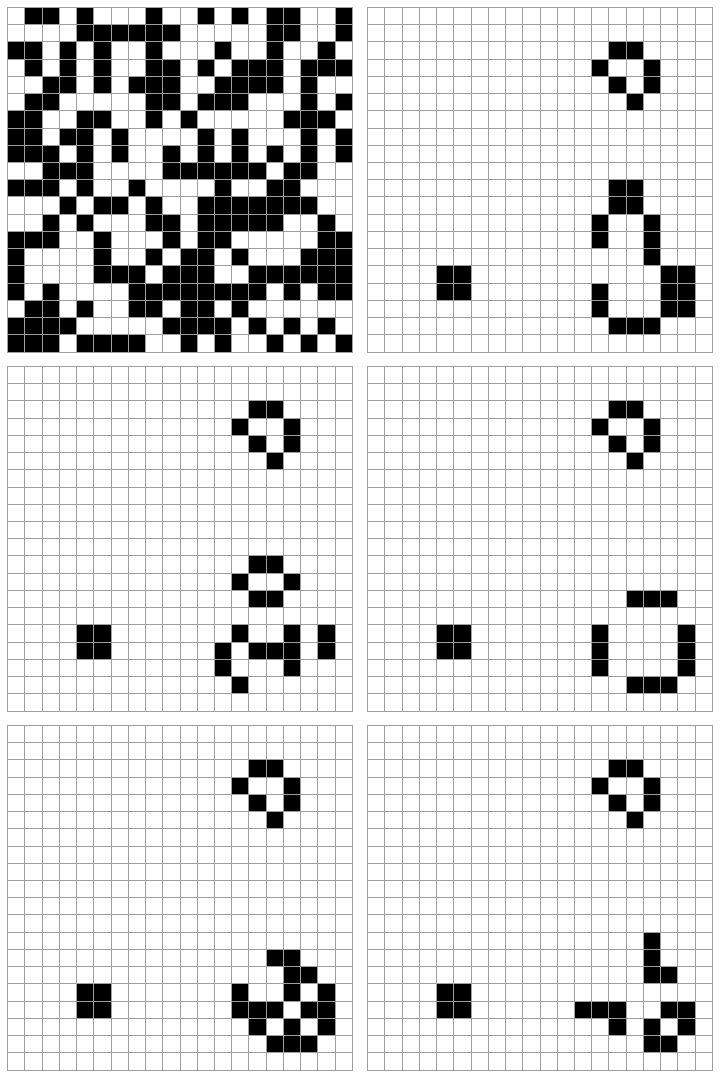
What a beauty. The initial chaos almost completely stabilizes after just a few iterations. We see that there exist stationary patterns, the 2×2 square in the bottom left and the space-invader in the top right. Finally, after the identity crisis in the bottom right flounders for a while, we get an oscillating pattern!

Now hold on, because we recognize that this oscillator (which we henceforth dub, the flame) is resting against the no man’s land. So it might not be genuine, and only oscillate because the edge allows it to. However, we notice that one of the patterns which precedes the flame is a 3×3 live square with a dead center. Let’s try putting this square by itself to see what happens. In order to do this, we have an extra few lines of code to transform a list of local coordinates to a pattern centered in a larger grid.

patternToGrid[pts_List, n_] :=
  With[{xOff = Floor[n/2] - Floor[Max[Map[#[[2]] &, pts]]/2],
        yOff = Floor[n/2] - Floor[Max[Map[#[[1]] &, pts]]/2]},
   SparseArray[Map[# + {yOff, xOff} -> 1 &, pts], {n, n}, 0]];
square = {{1, 1}, {1, 2}, {1, 3}, {2, 1}, {2, 3},
  {3, 1}, {3, 2}, {3, 3}};

Combining the resulting two lines with the earlier code for animation, we produce the following pattern:

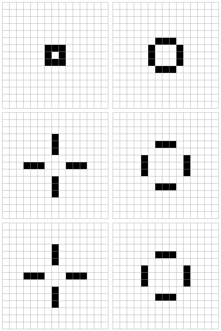
While we didn’t recover our coveted flame from before, we have at least verified that natural oscillators exist. It’s not hard to see that one of the four pieces above constitutes the smallest oscillator, for any oscillator requires at least three live cells in every generation, and this has exactly three in each generation. No less populated (static or moving) pattern could possibly exist indefinitely.

Before we return to our attempt to recreate the flame, let’s personify this animation. If we think of the original square as a densely packed community, we might tend to interpret this pattern as a migration. The packed population breaks up and migrates to form four separate communities, each of which is just the right size to sustain itself indefinitely. The astute reader may ask whether this is always the case: does every pattern dissipate into a stable pattern? Indeed, this was John Conway’s original question, and we will return to it in a moment.

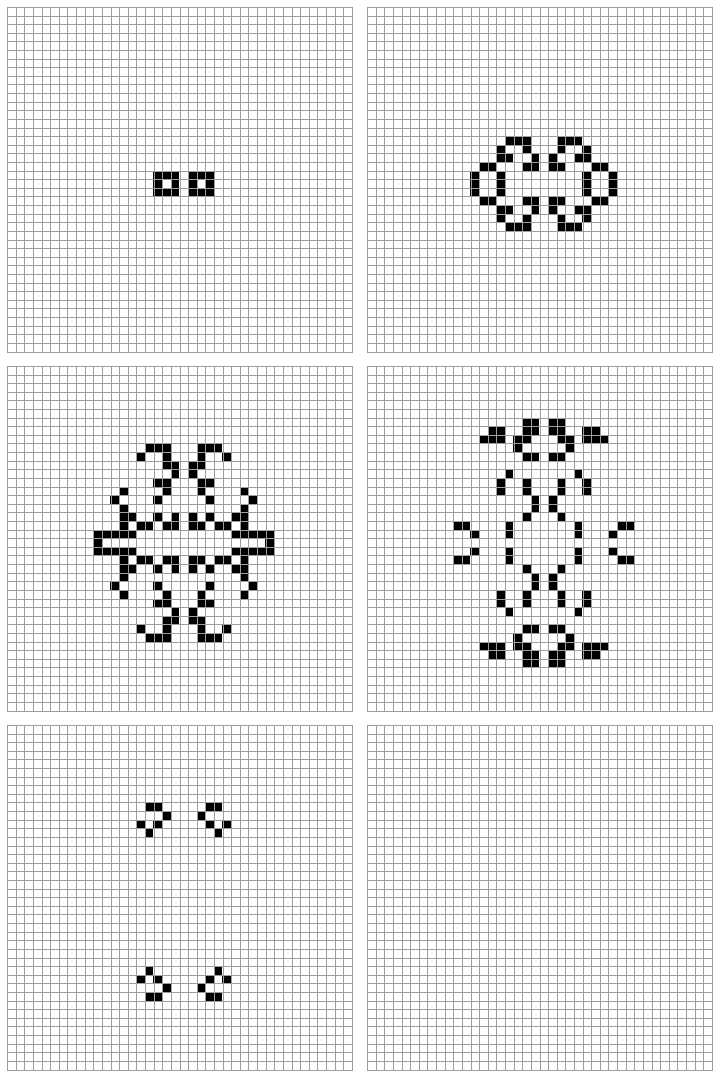
For now, we notice that the original square preceding the flame grew until its side hit a wall. Now we realize that the wall was essential in its oscillation. So, let us use the symmetry in the pattern to artificially create a “wall” in the form of another origin square. After a bit of tweaking to get the spacing right (three cells separating the squares), we arrive at the following unexpected animation:

With four symmetrically oscillating flames, it looks more like a jellyfish than a fire. But while we meant to produce two flames, we ended up with four! Quite marvelous. Here is another beautiful reject, which we got by placing the two squares only one cell apart. Unfortunately, it evaporates rather quickly. We call it, the fleeting butterfly.

We refrain from experimenting with other perturbations of the two-square initial configuration for the sake of completing this post by the end of the year. If the reader happens to find an interesting pattern, he shouldn’t hesitate to post a comment!

Now, before returning to the stabilization question, we consider one more phenomenon: moving patterns. Consider the following initial configuration:

A few mundane calculations show that in four generations this pattern repeats itself, but a few cells to the south-east. This glider pattern will fly indefinitely to its demise in no man’s land, as we see below.

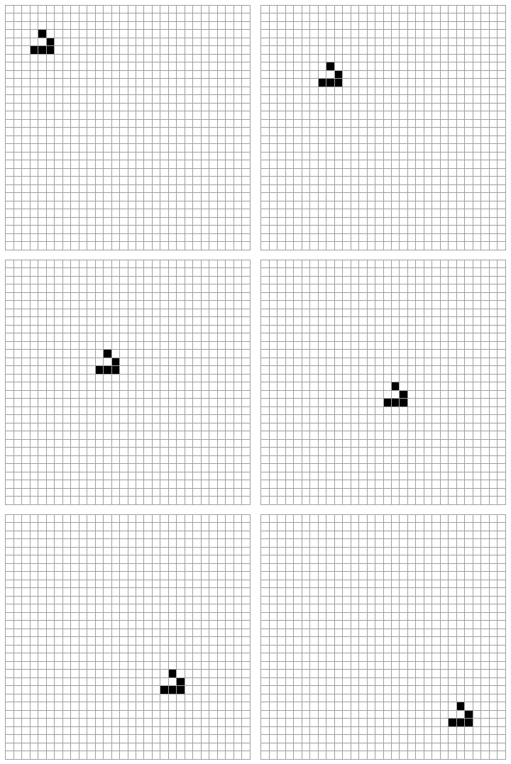
Awesome. And clearly, we can exploit the symmetry of this object to shoot the glider in all four directions. Let’s see what happens when they collide!

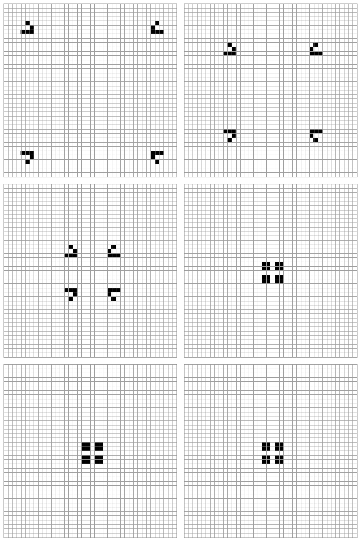
Well that was dumb. It’s probably too symmetric. We leave it as an exercise to the reader to slightly modify the initial position (given in the Mathematica notebook on this blog’s Github page) and witness the hopefully ensuing chaos.

Now you may have noticed that these designs are very pretty. Indeed, before the post intermission (there’s still loads more to explore), we will quickly investigate this idea.

Automata in Design

Using automata in design might seem rather far-fetched, and certainly would be difficult to implement (if not impossible) in an environment such as Photoshop or with CSS. But, recalling our post on Randomness in Design, it is only appropriate to show a real-world example of a design based on a cellular automaton (specifically, it seems to use something similar to rule 30 of the elementary automata). The prominent example at hand is the Conus seashell.

The Conus has cells which secrete pigment according to some unknown set of rules. That the process is a cellular automaton is stated but unsupported on Wikipedia. As unfortunate as that is, we may still appreciate that the final result looks like it was generated from a cellular automaton, and we can reproduce such designs with one. If I had more immediate access to a graphics library and had a bit more experience dealing with textures, I would gladly produce something. If at some point in the future I do get such experience, I would like to return to this topic and see what I can do. For the moment, however, we just admire the apparent connection.

A Tantalizing Peek

We have yet to breach the question of stabilization. In fact, though we started talking about models for computation, we haven’t actually computed anything besides pretty pictures yet! We implore the reader to have patience, and assert presciently that the question of stabilization comes first.

On one hand, we can prove that from any initial configuration Life always stabilizes, arriving at a state where cell population growth cannot continue. Alternatively, we could discover an initial configuration which causes unbounded population growth. The immature reader will notice that this mathematical object would not be very interesting if the former were the case, and so it is likely the latter. Indeed, without unbounded growth we wouldn’t be able to compute much! Before we actually find such a pattern, we realize that unbounded growth is possible in two different ways. First, a moving pattern (like the glider) may leave cells in its wake which do not disappear. Similarly, a stationary pattern may regularly emit moving patterns. Next time, we will give the canonical examples of such patterns, and show their use in turning Life into a model for computation. Finally, we have some additional ideas to spice Life up, but we will leave those as a surprise, defaulting to exclude them if they don’t pan out.

Until next time!