Google's Page Rank—The Final Product

Dangling Nodes and Non-Uniqueness

Recall where we left off last time. Given a web $ W$ with no dangling nodes, the link matrix for $ W$ has 1 as an eigenvalue, and if the corresponding eigenspace has dimension 1, then any associated eigenvector gives a ranking of the pages in $ W$ which is consistent with our goals.

The first problem is that if there is a dangling node, our link matrix has a column of all zeros, and is no longer column-stochastic. In fact, such a non-negative matrix which has columns summing to 1 or columns of all zeros is called column-substochastic. We cannot guarantee that 1 is an eigenvalue, with the obvious counterexample being the zero matrix.

Second, as we saw last time, webs which have disconnected subwebs admit eigenspaces of large dimension, and hence our derived rankings are not unique.

We will fix both of these problems in one fell swoop: by adjusting the link matrix to make all entries positive.

The motivation for this comes from the knowledge of a particular theorem, called the Perron-Frobenius Theorem. While the general statement says a great deal, here are the parts we need:

Theorem: Let $ A$ be a positive, column-stochastic matrix. Then there exists a maximal eigenvalue $ 0 < \lambda \leq 1$ such that all other eigenvalues are strictly smaller in magnitude. Further, the eigenspace associated to $ \lambda$ has dimension 1. This unique eigenvalue and eigenvector (up to scaling) are called the Perron eigenvalue and eigenvector.

We won’t prove this theorem, because it requires a lot of additional background. But we will use it to make life great. All we need is a positive attitude.

A Drunkard’s Surf

Any tinkering with the link matrix must be done in a sensible way. Unfortunately, we can’t “add” new links to our web without destroying its original meaning. So we need to view the resulting link matrix in a different light. Enter probability theory.

So say you’re drunk. You’re surfing the web and at every page you click a random link. Suppose further that every page is just a list of links, so it’s not harder to find some than others, and you’re equally likely to pick any link on the site. If you continue surfing for a long time, you’d expect to see pages with lots of backlinks more often than those with few backlinks. As you sober up, you might realize that this is a great way to characterize how important a webpage is! You quickly write down the probabilities for an example web into a matrix, with each $ i,j$ entry being the probability that you click on a link from page $ j$ to go to page $ i$.

This is a bit of drunken mathematical gold! We’ve constructed precisely the same link matrix for a web, but found from a different perspective. Unfortunately, after more surfing you end up on a page that has no links. You cannot proceed, so you randomly type in a URL into the address bar, and continue on your merry way. Soon enough, you realize that you aren’t seeing the same webpages as you did in the first walk. This random URL must have taken you to a different connected component of the web. Brilliant! Herein we have the solution to both of our problems: add in some factor of random jumping.

To do this, and yet maintain column-stochasticity, we need to proportionally scale the elements of our matrix. Let $ A$ be our original link matrix, and $ B$ be the $ n \times n$ matrix with all entries $ 1/n$. Then form a new matrix:

In words, $ C$ has a factor of egalitarianism proportional to $ p$. All we need to verify is that $ C$ is still column-stochastic, and this is clear since each column sum looks like the following for a fixed $ j$ (and $ a_{i,j}$ denotes the corresponding entry of $ A$):

So, applying the Perron-Frobenius theorem to our new matrix (where the value $ p$ becomes a parameter in need of tuning), there is a unique largest positive eigenvalue $ \lambda \leq 1$ for this web with an eigenspace of dimension 1. Picking any eigenvector within that eigenspace and then normalizing it to a unit vector with positive entries, we have our ranking algorithm!

Aside: note that the assumption that the eigenvalue has all positive entries is not unfounded. This follows as a result of our new matrix $ C$ being irreducible. The details of this implication are unnecessary, as the Perron-Frobenius theorem provides the positivity of the Perron eigenvector. Furthermore, all other eigenvectors (corresponding to any eigenvalues) must have an entry which is either negative or non-real. Hence, we only have one available eigenvector to choose for any valid ranking.

Computing the Beast

A link matrix for a web of any reasonable size is massive. As of June 20th, 2011, Google has an indexed database of close to 46 billion web pages, and in its infancy at Stanford, PageRank was tested on a web of merely 24 million pages. Clearly, one big matrix cannot fit in the memory of a single machine. But before we get to the details of optimizing for scale, let us compute page ranks for webs of modest sizes.

The problem of computing eigenvectors was first studied around the beginning of the 1900s. The first published method was called the power method, and it involves approximating the limit of the sequence

for some arbitrary initial starting vector $ v_0$. Intuitively, when we apply $ C$ to $ v$, it “pulls” $ v$ toward each of its eigenvectors proportionally to their associated eigenvalues. In other words, the largest eigenvalue dominates. So an element of this sequence which has a high index will have been pulled closer and closer to an eigenvector corresponding to the largest eigenvalue (in absolute value), and hence approximate that eigenvector. Since we don’t want our vector to grow arbitrarily in size, we normalize it at each step. A more detailed analysis exists which formalizes this concept, but we only need to utilize it.

Under a few assumptions this sequence is guaranteed to converge. Specifically, we require that the matrix is real-valued, there exists a dominant eigenvalue, and the starting vector has a nonzero component in the direction of an eigenvector corresponding to the dominant eigenvalue. Luckily for us, existence is taken care of by the Perron-Frobenius theorem, real-valuedness by construction, and we may trivially pick an initial vector of all 1s. Here is the pseudocode:

C <- link matrix
v <- (1,1,...,1)

while true:
   previous = v
   v = dot(C, v)
   v /= norm(v)
   break if norm(v-previous) < epsilon

return v

The only thing we have to worry about is the inefficiency in computing $ v = Cv$, when $ C$ is a matrix that is dense, in the sense that there are very few 0’s. That means computing $ Cv$ will take $ \Theta(n^2)$ multiplications, even though there are far fewer links in the original link matrix $ A$. For a reasonable web of 24 million pages, this is mind-bogglingly slow. So we will replace this line with its original derivation:

   v = (p/n)*v + (1-p)*dot(A,v)

With the recognition that there exist special algorithms for sparse matrix multiplication, this computation is much faster.

Finally, our choice of epsilon is important, because we have yet to speak of how fast this algorithm converges. According to the analysis (linked) above, we can say a lot more than big-O type runtime complexity. The sequence actually converges geometrically, in the sense that each $ v_k$ is closer to the limit than $ v_{k-1}$ by a factor of $ r, 0 < r < 1$, which is proven to be $ \frac{|\lambda_2|}{|\lambda_1|}$, the ratio of the second and first dominant eigenvalues. If $ \lambda_2$ is very close to $ \lambda_1$, then the method will converge slowly. However, according to the research done on PageRank, the value of $ r$ usually sits at about 0.85, making the convergence rather speedy. So picking reasonably small values of epsilon (say, $ 10^{-10}$) will not kill us.

Implementation

Of course, writing pseudocode is child’s play compared to actually implementing a real algorithm. For pedantic purposes we chose to write PageRank in Mathematica, which has some amazing visualization features for graphs and plots, and built-in computation rules for sparse matrix multiplication. Furthermore, Mathematica represents graphs as a single object, so we can have very readable code. You can download the entire Mathematica notebook presented here from this blog’s Github page.

The code for the algorithm itself is not even fifteen lines of code (though it’s wrapped here to fit). We make heavy use of the built in functions for manipulating graph objects, and you should read the Mathematica documentation on graphs for more detailed information. But it’s pretty self-explanatory, black-box type code.

rulesToPairs[i_ -> j_] := {i,j};
SetAttributes[rulesToPairs, Listable];

PageRank[graph_, p_] := Module[{v, n, prev, edgeRules, degrees,
                                linkMatrixRules, linkMatrix},
   edgeRules = EdgeRules[graph];
   degrees = VertexCount[graph];
   n = VertexCount[graph];

   (* setting up the sparse array as a list of rules *)
   linkMatrixRules =
      Table[{pt[[2]],pt[[1]]} -> 1/degrees[[pt[[1]]]]],
            {pt, rulesToPairs[edgeRules]}];
   linkMatrix = SparseArray[linkMatrixRules, {n, n}];

   v = Table[1.0, {n}];
   While[True,
      prev = v;
      v = (p/n) + (1-p)Dot[linkMatrix, v];
      v = v/Norm[v];
      If[Norm[v-prev] < 10^(-10), Break[]]
   ];

   Return[Round[N[v], 0.001]]
];

And now to test it, we simply provide it a graph object, which might look like

Graph[{1->2, 2->3, 3->4, 4->2, 4->1, 3->1, 2->4}]

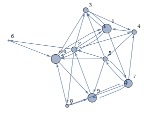
And it spits out the appropriate answer. Now, the output of PageRank is just a list of numbers between 0 and 1, and it’s not very easy to see what’s going on as you change the parameter $ p$. So we have some visualization code that gives very pretty pictures. In particular, we set the size of each vertex to be its page rank. Page rank values are conveniently within the appropriate range for the VertexSize option.

visualizePageRanks[G_, p_] := Module[{ranks},
   ranks = PageRank[G,p];
   Show[
     Graph[
      EdgeRules[G], 
      VertexSize -> Table[i -> ranks[[i]], {i, VertexCount[G]}],
      VertexLabels -> "Name",
      ImagePadding -> 10
     ]
   ]
];

And we have some random graphs to work with:

randomGraph[numVertices_, numEdges_] :=
  RandomGraph[{numVertices, numEdges},
              DirectedEdges -> True,
              VertexLabels -> "Name",
              ImagePadding -> 10]

Here’s the result for a random graph on 10 vertices and 30 edges, with $ p = 0.25$.

Furthermore, using Mathematica’s neat (but slow) commands for animation, we can see what happens as we vary the parameter $ p$ between zero and one:

Pretty neat!

Surprisingly enough (given that this is our first try implementing PageRank), the algorithm scales without issue. A web of ten-thousand vertices and thirty-thousand edges takes a mere four seconds on an Atom 1.6 GHz processor with a gig of RAM. Unfortunately (and this is where Mathematica starts to show its deficiencies) the RandomGraph command doesn’t support constructions of graphs with as few as 100,000 vertices and 200,000 edges. We leave it as an exercise to the reader to test the algorithm on larger datasets (hint: construct a uniformly distributed list of random rules, then count up the out-degrees of each vertex, and modify the existing code to accept these as parameters).

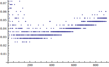
To give a better idea of how the algorithm works with respect to varying parameters, we have the following two graphs. The first is a runtime plot for random graphs where the number of vertices is fixed at 100 and the number of edges varies between 100 and 1000. Interestingly enough, the algorithm seems to run quickest when there are close to twice the number of edges as there are vertices.

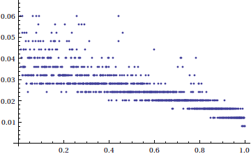
Next, we investigate the effects of varying $ p$, the egalitarianism factor, between 0 and 1 for random graphs with 100 vertices and 200 edges. Unsurprisingly, the runtime is fastest when we are completely egalitarian, and $ p$ is close to 1.

Google reportedly used $ p = 0.15$, so there probably were not significant gains in performance from the tuning of that parameter alone. Further, the structure of the web is not uniform; obviously there are large link hubs and many smaller sites which have relatively few links. With a bit more research into the actual density of links in the internet, we could do much better simulations. However, this sort of testing is beyond the scope of this blog.

So there you have it! A fully-functional implementation of PageRank, which scales as well as one could hope a prototype to. Feel free to play around with the provided code (assuming you don’t mind Mathematica, which is honestly a very nice language), and comment with your findings!

Next time we’ll wrap up this series with a discussion of the real-world pitfalls of PageRank. We will likely stray away from mathematics, but the consequences of such a high-profile ranking algorithm is necessary for completeness.

Page Rank Series

• An Introduction
• A First Attempt
• The Final Product
• Why It Doesn’t Work Anymore